从DDPM到DDIM(四) 预测噪声与后处理

前情回顾

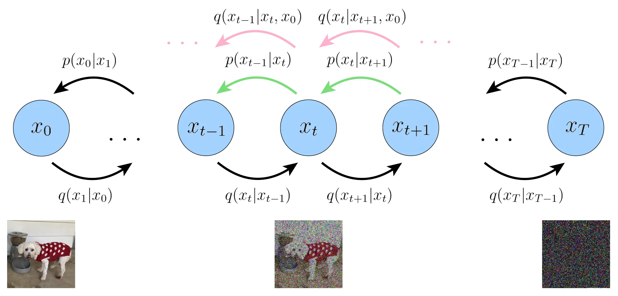
下图展示了DDPM的双向马尔可夫模型。

训练目标。最大化证据下界等价于最小化以下损失函数：

\[\boldsymbol{\theta}^*=\underset{\boldsymbol{\theta}}{\operatorname{argmin}} \sum_{t=1}^T \frac{1}{2 \sigma^2(t)} \frac{\left(1-\alpha_t\right)^2 \overline{\alpha}_{t-1}}{\left(1-\overline{\alpha}_t\right)^2} \mathbb{E}_{q\left(\mathbf{x}_t \mid \mathbf{x}_0\right)}\left[\Vert\tilde{\mathbf{x}}_{\boldsymbol{\theta}}\left(\mathbf{x}_t, t\right)-\mathbf{x}_0\Vert_2^2\right] \tag{1}

\]

推理过程。推理过程利用马尔可夫链蒙特卡罗方法。

\[\begin{aligned}

\mathbf{x}_{t-1} &\sim p_{\theta}\left(\mathbf{x}_{t-1} | \mathbf{x}_{t}\right) = \mathcal{N}(\mathbf{x}_{t-1}; \tilde{\bm{\mu}}_{\theta}\left(\mathbf{x}_{t}, t\right) , \sigma^2 \left(t\right) \mathbf{I}) \\

\mathbf{x}_{t-1} &= \tilde{\bm{\mu}}_{\theta}\left(\mathbf{x}_{t}, t\right) + \sigma \left(t\right) \bm{\epsilon} \\

&= \frac{\left( 1 - \overline{\alpha}_{t-1} \right) \sqrt{\alpha_t}}{\left( 1 - \overline{\alpha}_{t} \right)} \mathbf{x}_{t} + \frac{\left(1 - \alpha_t\right) \sqrt{\overline{\alpha}_{t-1}}}{\left( 1 - \overline{\alpha}_{t} \right)} \tilde{\mathbf{x}}_{\theta} \left(\mathbf{x}_{t}, t\right) + \sigma \left(t\right) \bm{\epsilon}

\end{aligned} \tag{2}

\]

1、预测噪声

上一篇文章我们提到，扩散模型的神经网络用于预测 \(\mathbf{x}_{0}\)，然而DDPM并不是这样做的，而是用神经网络预测噪声。这也是DDPM 第一个字母 D(Denoising)的含义。为什么采用预测噪声的参数化方法？DDPM作者在原文中提到去噪分数匹配(denoising score matching, DSM)，并说这样训练和DSM是等价的。可见应该是收了DSM的启发。另外一个解释我们一会来讲。

按照上一篇文章的化简技巧，对于神经网络的预测输出 \(\tilde{\mathbf{x}}_{\boldsymbol{\theta}}\left(\mathbf{x}_t, t\right)\)，也可以进行进一步参数化(parameterization)：

已知：

\[\begin{aligned}

\mathbf{x}_{t} = \sqrt{\overline{\alpha}_t} \mathbf{x}_{0} + \sqrt{1 - \overline{\alpha}_t} \bm{\epsilon}

\end{aligned} \tag{3}

\]

于是：

\[\begin{aligned}

\mathbf{x}_{0} = \frac{1}{\sqrt{\overline{\alpha}_t}} \mathbf{x}_{t} + \frac{\sqrt{1 - \overline{\alpha}_t}}{\sqrt{\overline{\alpha}_t}} \bm{\epsilon}

\end{aligned} \tag{4}

\]

\[\begin{aligned}

\tilde{\mathbf{x}}_{\boldsymbol{\theta}}\left(\mathbf{x}_t, t\right) = \frac{1}{\sqrt{\overline{\alpha}_t}} \mathbf{x}_{t} + \frac{\sqrt{1 - \overline{\alpha}_t}}{\sqrt{\overline{\alpha}_t}} \tilde{\bm{\epsilon}}_{\boldsymbol{\theta}}\left(\mathbf{x}_t, t\right)

\end{aligned} \tag{5}

\]

这里我们解释以下为什么采用预测噪声的方式的第二个原因。从(4)(5)两式可见，噪声项可以看作是 \(\mathbf{x}_{0}\) 与 \(\mathbf{x}_{t}\) 的残差项。回顾经典的Resnet结构：

\[\left[\mathbf{y}=\mathbf{x}+\mathcal{F}\left(\mathbf{x}, W_i\right)\right]

\]

Resnet也是用神经网络学习的残差项。DDPM采用预测噪声的方法和Resnet残差学习由异曲同工之妙。

下面我们将(3)(4)两式代入(1)式，继续化简，有：

\[\begin{aligned}

\Vert\tilde{\mathbf{x}}_{\boldsymbol{\theta}}\left(\mathbf{x}_t, t\right)-\mathbf{x}_0\Vert_2^2 &= \frac{1 - \overline{\alpha}_t}{\overline{\alpha}_t} \Vert\tilde{\bm{\epsilon}}_{\boldsymbol{\theta}}\left(\mathbf{x}_t, t\right)-\bm{\epsilon}\Vert_2^2

\end{aligned}

\]

注意 \(\overline{\alpha}_t\) = \(\overline{\alpha}_{t-1} \alpha_t\)于是可以得出新的优化方程：

\[\boldsymbol{\theta}^*=\underset{\boldsymbol{\theta}}{\operatorname{argmin}} \sum_{t=1}^T \frac{1}{2 \sigma^2(t)} \frac{\left(1-\alpha_t\right)^2}{\left(1-\overline{\alpha}_t\right) \alpha}_t \mathbb{E}_{q\left(\mathbf{x}_t \mid \mathbf{x}_0\right)}\left[\Vert\tilde{\bm{\epsilon}}_{\boldsymbol{\theta}}\left(\sqrt{\overline{\alpha}_t} \mathbf{x}_{0} + \sqrt{1 - \overline{\alpha}_t} \bm{\epsilon}, t\right)-\bm{\epsilon}\Vert_2^2\right] \tag{6}

\]

(6) 式表示，我们的神经网络 \(\tilde{\bm{\epsilon}}_{\boldsymbol{\theta}}\left(\sqrt{\overline{\alpha}_t} \mathbf{x}_{0} + \sqrt{1 - \overline{\alpha}_t} \bm{\epsilon}, t\right)\) 被用于预测最初始的噪声 \(\bm{\epsilon}\)。忽略掉前面的系数，对应的训练算法如下：

Algorithm 3 . Training a Deniosing Diffusion Probabilistic Model. (Version: Predict noise)

Repeat the following steps until convergence.

• For every image \(\mathbf{x}_0\) in your training dataset \(\mathbf{x}_0 \sim q\left(\mathbf{x}_0\right)\)
• Pick a random time step \(t \sim \text{Uniform}[1, T]\).
• Generate normalized Gaussian random noise \(\bm{\epsilon} \sim \mathcal{N} \left(\mathbf{0}, \mathbf{I}\right)\)
• Take gradient descent step on

\[\nabla_{\boldsymbol{\theta}} \Vert\tilde{\bm{\epsilon}}_{\boldsymbol{\theta}}\left(\sqrt{\overline{\alpha}_t} \mathbf{x}_{0} + \sqrt{1 - \overline{\alpha}_t} \bm{\epsilon}, t\right)-\bm{\epsilon}\Vert_2^2

\]

You can do this in batches, just like how you train any other neural networks. Note that, here, you are training one denoising network \(\tilde{\bm{\epsilon}}_{\boldsymbol{\theta}}\) for all noisy conditions.

推理的过程依然从马尔可夫链蒙特卡洛(MCMC)开始，因为这里是预测噪声，而推理的过程中也需要加噪声，为了区分，我们将推理过程中添加的噪声用 \(\mathbf{z} \sim \mathcal{N} \left(\mathbf{0}, \mathbf{I}\right)\) 来表示。推理过程中每次推理的噪声 \(\mathbf{z}\) 都是不同的，但训练过程中要拟合的最初的目标噪声 \(\bm{\epsilon}\) 是相同的。

\[\begin{aligned}

\mathbf{x}_{t-1} &\sim p_{\theta}\left(\mathbf{x}_{t-1} | \mathbf{x}_{t}\right) = \mathcal{N}(\mathbf{x}_{t-1}; \tilde{\bm{\mu}}_{\theta}\left(\mathbf{x}_{t}, t\right) , \sigma^2 \left(t\right) \mathbf{I}) \\

\mathbf{x}_{t-1} &= \tilde{\bm{\mu}}_{\theta}\left(\mathbf{x}_{t}, t\right) + \sigma \left(t\right) \mathbf{z} \\

&= \frac{\left( 1 - \overline{\alpha}_{t-1} \right) \sqrt{\alpha_t}}{\left( 1 - \overline{\alpha}_{t} \right)} \mathbf{x}_{t} + \frac{\left(1 - \alpha_t\right) \sqrt{\overline{\alpha}_{t-1}}}{\left( 1 - \overline{\alpha}_{t} \right)} \tilde{\mathbf{x}}_{\theta} \left(\mathbf{x}_{t}, t\right) + \sigma \left(t\right) \mathbf{z}

\end{aligned} \tag{7}

\]

将(5)式代入：

\[\begin{aligned}

\tilde{\bm{\mu}}_{\theta}\left(\mathbf{x}_{t}, t\right) &= \frac{\left( 1 - \overline{\alpha}_{t-1} \right) \sqrt{\alpha_t}}{\left( 1 - \overline{\alpha}_{t} \right)} \mathbf{x}_{t} + \frac{\left(1 - \alpha_t\right) \sqrt{\overline{\alpha}_{t-1}}}{\left( 1 - \overline{\alpha}_{t} \right)} \tilde{\mathbf{x}}_{\theta} \left(\mathbf{x}_{t}, t\right) \\

&= \frac{\left( 1 - \overline{\alpha}_{t-1} \right) \sqrt{\alpha_t}}{\left( 1 - \overline{\alpha}_{t} \right)} \mathbf{x}_{t} + \frac{\left(1 - \alpha_t\right) \sqrt{\overline{\alpha}_{t-1}}}{\left( 1 - \overline{\alpha}_{t} \right)} \left( \frac{1}{\sqrt{\overline{\alpha}_t}} \mathbf{x}_{t} + \frac{\sqrt{1 - \overline{\alpha}_t}}{\sqrt{\overline{\alpha}_t}} \tilde{\bm{\epsilon}}_{\boldsymbol{\theta}}\left(\mathbf{x}_t, t\right) \right) \\

&= \text{some algebra calculation} \\

&= \frac{1}{\sqrt{\overline{\alpha}_t}} \mathbf{x}_{t} + \frac{1 - \alpha_t}{ \sqrt{ \left( 1 - \overline{\alpha}_{t} \right)\alpha}_t} \tilde{\bm{\epsilon}}_{\boldsymbol{\theta}}\left(\mathbf{x}_t, t\right)

\end{aligned}

\]

所以推理的表达式为：

\[\begin{aligned}

\mathbf{x}_{t-1} &= \frac{1}{\sqrt{\overline{\alpha}_t}} \mathbf{x}_{t} + \frac{1 - \alpha_t}{ \sqrt{ \left( 1 - \overline{\alpha}_{t} \right)\alpha}_t} \tilde{\bm{\epsilon}}_{\boldsymbol{\theta}}\left(\mathbf{x}_t, t\right) + \sigma \left(t\right) \mathbf{z}

\end{aligned} \tag{7}

\]

下面可以写出采用拟合噪声策略的推理算法：

Algorithm 4 . Inference on a Deniosing Diffusion Probabilistic Model. (Version: Predict noise)

You give us a white noise vector \(\mathbf{x}_T \sim \mathcal{N} \left(\mathbf{0}, \mathbf{I}\right)\)

Repeat the following for \(t = T, T − 1, ... , 1\).

• Generate \(\mathbf{z} \sim \mathcal{N} \left(\mathbf{0}, \mathbf{I}\right)\) if \(t > 1\) else \(\mathbf{z} = \mathbf{0}\)

\[\mathbf{x}_{t-1} = \frac{1}{\sqrt{\overline{\alpha}_t}} \mathbf{x}_{t} + \frac{1 - \alpha_t}{ \sqrt{ \left( 1 - \overline{\alpha}_{t} \right)\alpha}_t} \tilde{\bm{\epsilon}}_{\boldsymbol{\theta}}\left(\mathbf{x}_t, t\right) + \sigma \left(t\right) \mathbf{z}

\]

Return \(\mathbf{x}_{0}\)

2、后处理

首先要注意到，在推理算法的最后一步，生成图像的时候，并没有添加噪声，而是直接采用预测的均值作为 \(\mathcal{x}_0\) 的估计值。

另外，生成的图像原本是归一化到 \([-1, 1]\) 之间的，所以要反归一化到 \([0, 255]\)。这里比较简单，直接看 diffusers 库中的代码：

<code>

image = (image / 2 + 0.5).clamp(0, 1)

image = image.cpu().permute(0, 2, 3, 1).numpy()

if output_type == "pil":

image = self.numpy_to_pil(image)

if not return_dict:

return (image,)

def numpy_to_pil(images):

"""

Convert a numpy image or a batch of images to a PIL image.

"""

if images.ndim == 3:

images = images[None, ...]

images = (images * 255).round().astype("uint8")

if images.shape[-1] == 1:

# special case for grayscale (single channel) images

pil_images = [Image.fromarray(image.squeeze(), mode="L") for image in images]code>

else:

pil_images = [Image.fromarray(image) for image in images]

return pil_images

3、总结

我们最初的目标是估计图像的概率分布，采用极大似然估计法，求 \(\log p\left(\mathbf{x}_0\right)\)。但是直接求解，很难求：

\[\begin{aligned}

p\left(\mathbf{x}_0\right) = \int p\left(\mathbf{x}_{0:T}\right) d \mathbf{x}_{1:T} \\

\end{aligned} \\

\]

而且 \(p\left(\mathbf{x}_{0:T}\right)\) 也不知道。于是我们选择估计它的证据下界。在计算证据下界的过程中，我们解析了双向马尔可夫链中的很多分布和变量，最终推导出证据下界的表达式，以KL散度的方式来表示。这样做本质上是用已知的分布 \(q\left(\mathbf{x}_{1:T} | \mathbf{x}_{0}\right)\) 来对未知的分布做逼近。这其实是 变分推断 的思想。变分法是寻找一个函数使得这个函数最能满足条件，而变分推断是寻找一个分布使之更加逼近已知的分布。

于是我们而在高斯分布的假设下，KL散度恰好等价于二范数的平方。最大似然估计等价于最小化二范数loss。之后就顺理成章地推导出了训练方法，并根据马尔可夫链蒙特卡洛推导出推理算法。关于变分推断和马尔可夫链蒙特卡洛相关的知识，读者可以自行查找，有时间我也会写篇文章来介绍。

以上就是DDPM的全部内容了，我用了四篇文章对DDPM进行了详细推导，写文章的过程中也弄懂了自己之前不懂的一些细节。我的最大的感受是，初学者千万不要相信诸如《一文读懂DDPM》之类的文章，如果要真正搞懂DDPM，只有自己把所有公式手推一边才是正道。

下一篇我们开始介绍DDPM的一个经典的推理加速方法：DDIM